Phase field fracture: Towards a generic method to follow the equilibrium path of the structure

Congrès des Jeunes Chercheurs en Mécanique

F. Loiseau

IMSIA, ENSTA Paris, CNRS, EDF, Institut Polytechnique de Paris 91120 Palaiseau, France

August 28, 2024

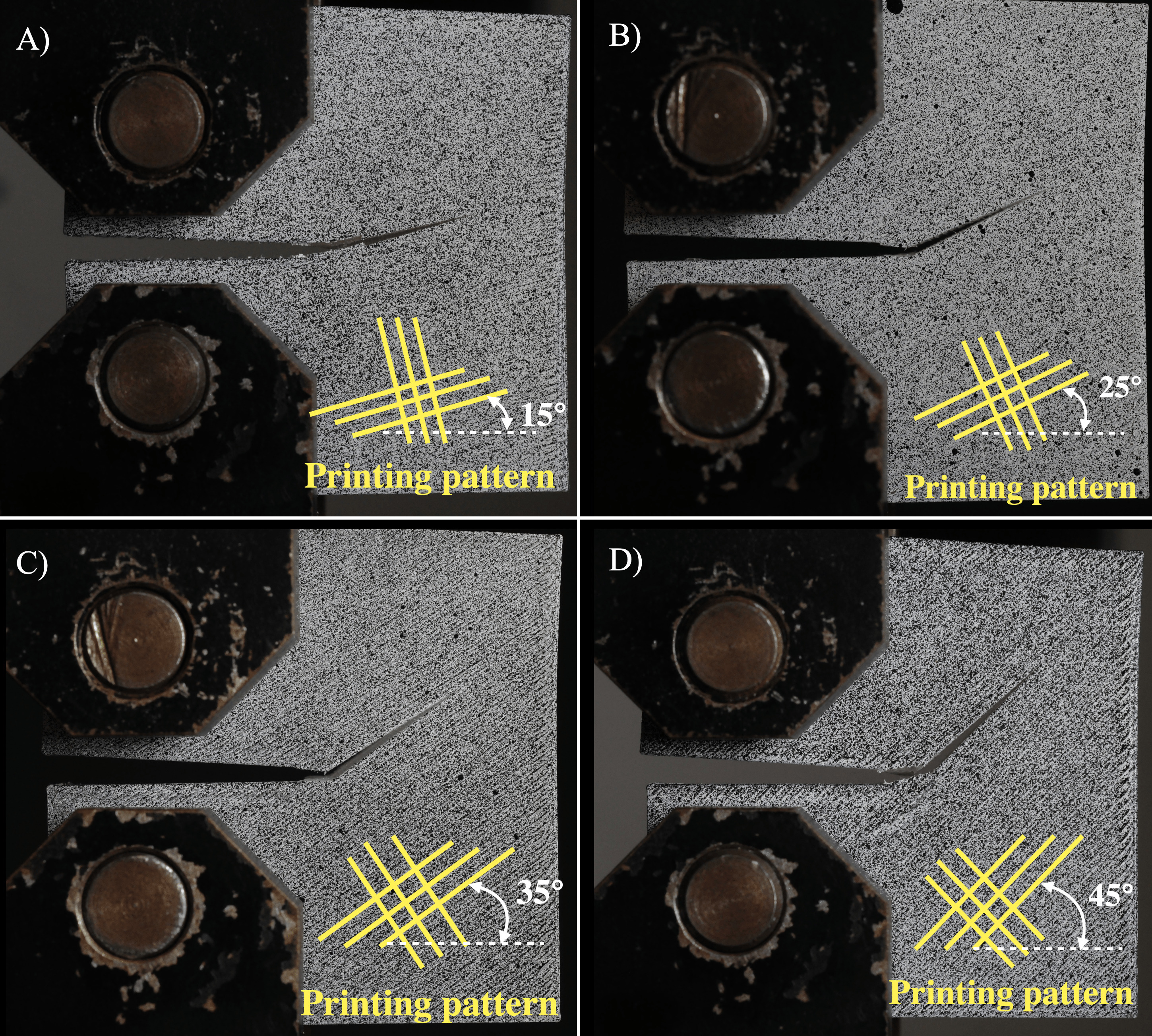
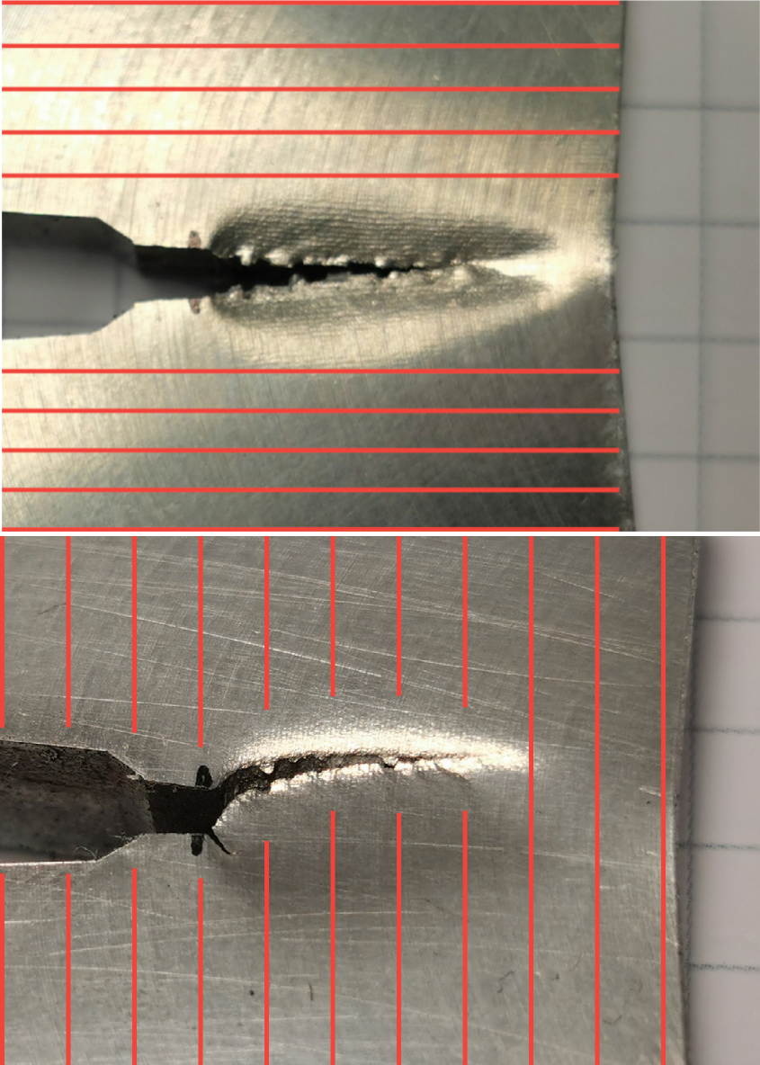
Fracture in 3D-printed structures

Polycarbonate CT specimen by FDM (Zhai, 2023)

Duplex stainless steel by DED (Roucou et al., 2023)

Global objective

Modelling and simulating crack propagation in 3D-printed structures

Fracture mechanics problem

We consider

  • a domain \(\Omega\) with a pre-crack \(\Gamma_0\),
  • an elastic material (\(E\), \(\nu\)),
  • a force or displacement load,

and we want to determine

  • the crack-path,
  • the force-displacement curve,
  • the evolution of the displacement field.

To solve this problem, we want to employ numerical methods.

Phase-field fracture

The state of a domain \(\Omega\) is described by:

  • a displacement field \(\boldsymbol{u}(\boldsymbol{x})\),
  • a crack phase field \(\alpha(\boldsymbol{x})\).

The state fields are governed by an energy minization problem, \[ (\boldsymbol{u}, \alpha) = \arg\min_{\substack{\boldsymbol{u}^* \in \mathcal{U} \\ \alpha^* \in \mathcal{A}}} \ \underset{\text{elastic}}{\mathcal{E} (\boldsymbol{u}^*, \alpha^*)} + \underset{\text{dissipation}}{\mathcal{D} (\alpha^*)} - \underset{\text{external work}}{\mathcal{W}_{\mathrm{ext}} (\boldsymbol{u}^*)} \]

Issues due to fracture (displacement loading)


Issue due to fracture (force loading)


Path-following methods 1

Principle

A load factor \(\lambda\) with a control equation,

\[ f(\lambda, \boldsymbol{u}, ...) - \Delta \tau= 0, \]

where \(\Delta \tau\): step size of control quantity \(f\).


From geometrical non-linearities

Wempner (1971), Riks (1972), Riks (1979),
Crisfield (1981), Ramm (1981).

Applications to phase-field fracture

Energy release/Dissipation
Gutiérrez (2004)

Application to phase-field fracture by

Pros

  • Problem-independent

Cons

  • Model-depend (dissipation)
  • Control switch for elastic phase

Nodal displacement
De Borst (1987)

Applied to phase-field by


Pros

  • Model-independent

Cons

  • A-priori choice of control nodes
    • Problem-depend

Can we introduce path-following in simulations of phase-field fracture?

With some constraints:

  • Simplicity (minimize intrusivity, no switch).
  • Flexibility (no model dependency, no problem dependency).
  • Robustness (no mesh dependency, no divergence).

Control equation

Control by Maximum Strain Increment (Chen & Schreyer, 1990)

The idea is to limit the maximum strain variation in the domain using the equation \[ \max_{\boldsymbol{x}\in \Omega} \left( \frac{\boldsymbol{\varepsilon}(\boldsymbol{u}_{n-1})}{\| \boldsymbol{\varepsilon}(\boldsymbol{u}_{n-1}) \|} : {\color{\red}\Delta \boldsymbol{\varepsilon}(\boldsymbol{u})} \right) - \Delta \tau= 0, \]

where \(\Delta \tau\) is the step size.

Solving the problem (alternate minimization)

Applications

SENT specimen: Presentation

SENT specimen: Displacement control

SENT specimen: Path-following control

CT specimen with force boundary conditions

Conclusion

We applied a path-following method based on control by maximum strain increment.

It proved to be:

  • simple: small changes to the elastic solver, none to the crack-phase solver.
  • flexible: no problem nor model dependencies.

Yet, we observed some divergence of the resolution in some specific cases.

Thank you for your attention !

F. Loiseau, V. Lazarus

flavien.loiseau@ensta-paris.fr

References

References

Chen, Z., & Schreyer, H. L. (1990). A numerical solution scheme for softening problems involving total strain control. Computers & Structures, 37(6), 1043–1050. https://doi.org/10.1016/0045-7949(90)90016-U
Crisfield, M. A. (1981). A fast incremental/iterative solution procedure that handles “snap-through.” Computers & Structures, 13(1), 55–62. https://doi.org/10.1016/0045-7949(81)90108-5
De Borst, R. (1987). Computation of post-bifurcation and post-failure behavior of strain-softening solids. Computers & Structures, 25(2), 211–224. https://doi.org/10.1016/0045-7949(87)90144-1
Gutiérrez, M. A. (2004). Energy release control for numerical simulations of failure in quasi-brittle solids. Communications in Numerical Methods in Engineering, 20(1), 19–29. https://doi.org/10.1002/cnm.649
Lorentz, E., & Badel, P. (2004). A new path-following constraint for strain-softening finite element simulations. International Journal for Numerical Methods in Engineering, 60(2), 499–526. https://doi.org/10.1002/nme.971
May, S., Vignollet, J., & Borst, R. de. (2016). A new arc-length control method based on the rates of the internal and the dissipated energy. Engineering Computations, 33(1), 100–115. https://doi.org/10.1108/EC-02-2015-0044
Ramm, E. (1981). Strategies for Tracing the Nonlinear Response Near Limit Points. In W. Wunderlich, E. Stein, & K.-J. Bathe (Eds.), Nonlinear Finite Element Analysis in Structural Mechanics (pp. 63–89). Springer. https://doi.org/10.1007/978-3-642-81589-8_5
Riks, E. (1972). The Application of Newton’s Method to the Problem of Elastic Stability. Journal of Applied Mechanics, 39(4), 1060–1065. https://doi.org/10.1115/1.3422829
Riks, E. (1979). An incremental approach to the solution of snapping and buckling problems. International Journal of Solids and Structures, 15(7), 529–551. https://doi.org/10.1016/0020-7683(79)90081-7
Roucou, D., Corre, T., Rolland, G., & Lazarus, V. (2023). Effect of the deposition direction on fracture propagation in a Duplex Stainless Steel manufactured by Directed Energy Deposition. Materials Science and Engineering: A, 878, 145176. https://doi.org/10.1016/j.msea.2023.145176
Singh, N., Verhoosel, C. V., Borst, R. de, & Brummelen, E. H. van. (2016). A fracture-controlled path-following technique for phase-field modeling of brittle fracture. Finite Elements in Analysis and Design, 113, 14–29. https://doi.org/10.1016/j.finel.2015.12.005
Wempner, G. A. (1971). Discrete approximations related to nonlinear theories of solids. International Journal of Solids and Structures, 7(11), 1581–1599. https://doi.org/10.1016/0020-7683(71)90038-2
Wu, J.-Y. (2018). Robust numerical implementation of non-standard phase-field damage models for failure in solids. Computer Methods in Applied Mechanics and Engineering, 340, 767–797. https://doi.org/10.1016/j.cma.2018.06.007
Zhai, X. (2023). Crack propagation in elastic media with anisotropic fracture toughness: Experiments and phase-field modeling [PhD thesis].

Appendices

Systematic literature review

Query

Search on Scopus using the following query in April, 2024.

("load control" OR "path following" OR "path-following" OR "arc length" OR "arc-length" OR "continuation")
AND ("phase-field")
AND ("fracture")

Results

  • 15 articles
  • 2 filtered out
    • 1 written in chinese
    • 1 unrelated
  • 2 added articles (not in the search, found by previous researches)

Notes

  • Main contributors at TU Delft
  • Few load control methods applied to PF
  • Various solving algorithm (staggered/monolithic)
  • Small/No comparison to LEFM
  • No comparison to expe

Phase-field fracture

The state of a domain \(\Omega\) is described by:

  • a displacement field \(\boldsymbol{u}(\boldsymbol{x})\)
  • a crack phase field \(\alpha(\boldsymbol{x})\)

The state of the domain verifies \[ (\boldsymbol{u}, \alpha) = \arg\min_{\substack{\boldsymbol{u}^* \in \mathcal{U} \\ \alpha^* \in \mathcal{A}}} \mathcal{E}_{\mathrm{tot}} = \arg\min_{\substack{\boldsymbol{u}^* \in \mathcal{U} \\ \alpha^* \in \mathcal{A}}} \mathcal{E} (\boldsymbol{u}^*, \alpha^*) + \mathcal{D} (\alpha^*) - \mathcal{W}_{\mathrm{ext}} (\boldsymbol{u}^*) \]

where the energy functionals are,

\[ \begin{split} \mathcal{E} (\boldsymbol{u}, \alpha) &= \int_{\Omega} \frac{1}{2} a(\alpha) \boldsymbol{\varepsilon}(\boldsymbol{u}) : \mathbf{E}: \boldsymbol{\varepsilon}(\boldsymbol{u}) \,\mathrm{d}x, \\ \mathcal{D} (\alpha) &= \int_{\Omega} \frac{G_c}{c_w} \left( \frac{w(\alpha)}{\ell} + \ell \nabla \alpha \cdot \nabla \alpha \right) \,\mathrm{d}x, \\ \mathcal{W} (\boldsymbol{u}) &= \int_{\partial \Omega} \lambda \boldsymbol{t}_{\mathrm{ctrl}}\cdot \boldsymbol{u}^* \,\mathrm{d}x. \end{split} \]

Staggered scheme (alternate minimization)


The minimization problem can be solved by splitting the problem into two subproblems:

  • minimization with respect to the displacement field \(\boldsymbol{u}(\boldsymbol{x})\) \[ \boldsymbol{u}(\boldsymbol{x}) = \arg\min_{\boldsymbol{u}^* \in \mathcal{U}} \mathcal{E}_{\mathrm{tot}} (\boldsymbol{u}^*, \alpha), \]
  • minimization of the functional with respect to the crack phase field \(\alpha(\boldsymbol{x})\) \[ \alpha(\boldsymbol{x}) =\arg\min_{\alpha^* \in \mathcal{A}} \mathcal{E}_{\mathrm{tot}} (\boldsymbol{u}, \alpha^*). \]

We need to introduce the solving of the control equation.

Solving procedure (displacement + load factor)

  1. Solve the displacement field \(\bar{\boldsymbol{u}}\) associated with a unitary load (\(\lambda = 1\))

\[ \begin{split} \forall \boldsymbol{v}\in \mathcal{U}_0, \quad & \int_{\Omega} a(\alpha) \boldsymbol{\varepsilon}(\bar{\boldsymbol{u}}) : \mathbf{E}: \boldsymbol{\varepsilon}(\boldsymbol{v}) \,\mathrm{d}x + \int_{\partial \Omega} \boldsymbol{t}_{\mathrm{ctrl}}\cdot \boldsymbol{v}\,\mathrm{d}x = 0, \end{split} \]

  1. Solve the control equation for each \(\boldsymbol{x}\in \Omega\) with \[ \frac{\boldsymbol{\varepsilon}(\boldsymbol{u}_{n-1})}{\| \boldsymbol{\varepsilon}(\boldsymbol{u}_{n-1}) \|} : \overbrace{({\color{\red}\lambda(\boldsymbol{x})} \boldsymbol{\varepsilon}(\boldsymbol{u}_{n-1}) - \boldsymbol{\varepsilon}(\boldsymbol{u}_{n-1}))}^{\Delta \boldsymbol{\varepsilon}(\boldsymbol{u})} - \Delta \tau= 0 \iff \lambda(\boldsymbol{x}) = \frac{\Delta \tau- a_0}{a_1}, \] where \(a_0 = \frac{\boldsymbol{\varepsilon}_{n-1} (\boldsymbol{x})}{\| \boldsymbol{\varepsilon}_{n-1}(\boldsymbol{x}) \|} : \boldsymbol{\varepsilon}_{n-1}(\boldsymbol{x})\), and \(a_1 = \frac{\boldsymbol{\varepsilon}_{n-1} (\boldsymbol{x})}{\| \boldsymbol{\varepsilon}_{n-1}(\boldsymbol{x}) \|} : \boldsymbol{\varepsilon}(\bar{\boldsymbol{u}})\).

  2. Select the load factor using the nested interval algorithm (Lorentz & Badel, 2004).

  3. Calculate the displacement field \(\boldsymbol{u}(\boldsymbol{x}) = \lambda \bar{\boldsymbol{u}}(\boldsymbol{x})\).